Tutorial
In this tutorial, we demonstrate the usage of the PicardLefschetzIntegration.jl.
Fresnel integral
Let us first consider the Fresnel integral
\[I = \int_{-\infty}^\infty e^{i x^2}\mathrm{d}x = (1+i)\sqrt{\frac{\pi}{2}}\]
The integral has a single critical point at $x = 0$. The associated Lefschetz thimble is the diagonal contour
\[\mathcal{J}=(1+i)\mathbb{R}.\]
using PicardLefschetzIntegration, CairoMakie, Makie.GeometryBasics

function linePlot(S, thim::thimble)
    filter!(sim->sim.active, thim.simplices)
    lines = reduce(vcat, [[Point2f(real(thim.points[i].coord[1]), imag(thim.points[i].coord[1])) for i in sim.coord] for sim in thim.simplices])
    vertices = stack(map(p -> p.coord, thim.points), dims=1)

    fig = Figure()
    ax = Axis(fig[1, 1], aspect=1)

    us, vs = LinRange(-5, 5, 100), LinRange(-4, 4, 100)
    h = [real(im * S([u + im * v])) for u in us, v in vs]

    heatmap!(ax, us, vs, h)

    contour!(ax, us, vs, h, color=:black, levels=20)

    linesegments!(ax, lines, linewidth=2, color=:red)

    scatter!(ax, real.(vertices[:]), imag.(vertices[:]))

    for i in 1:length(thim.points)
        text!(ax, real(vertices[i]), imag(vertices[i]) + 0.2, text = string(i))
    end
    limits!(ax, -5, 5, -4, 4)
    return fig
end

pars = parameters(δ = 0.5, τ = -10., ϵ = 0.1, N = 20, n = 5, dim = 1)

thim = initialGrid([-4], [4], pars)
S(p) = p[1]^2
flow!(S, thim, pars)
linePlot(S, thim)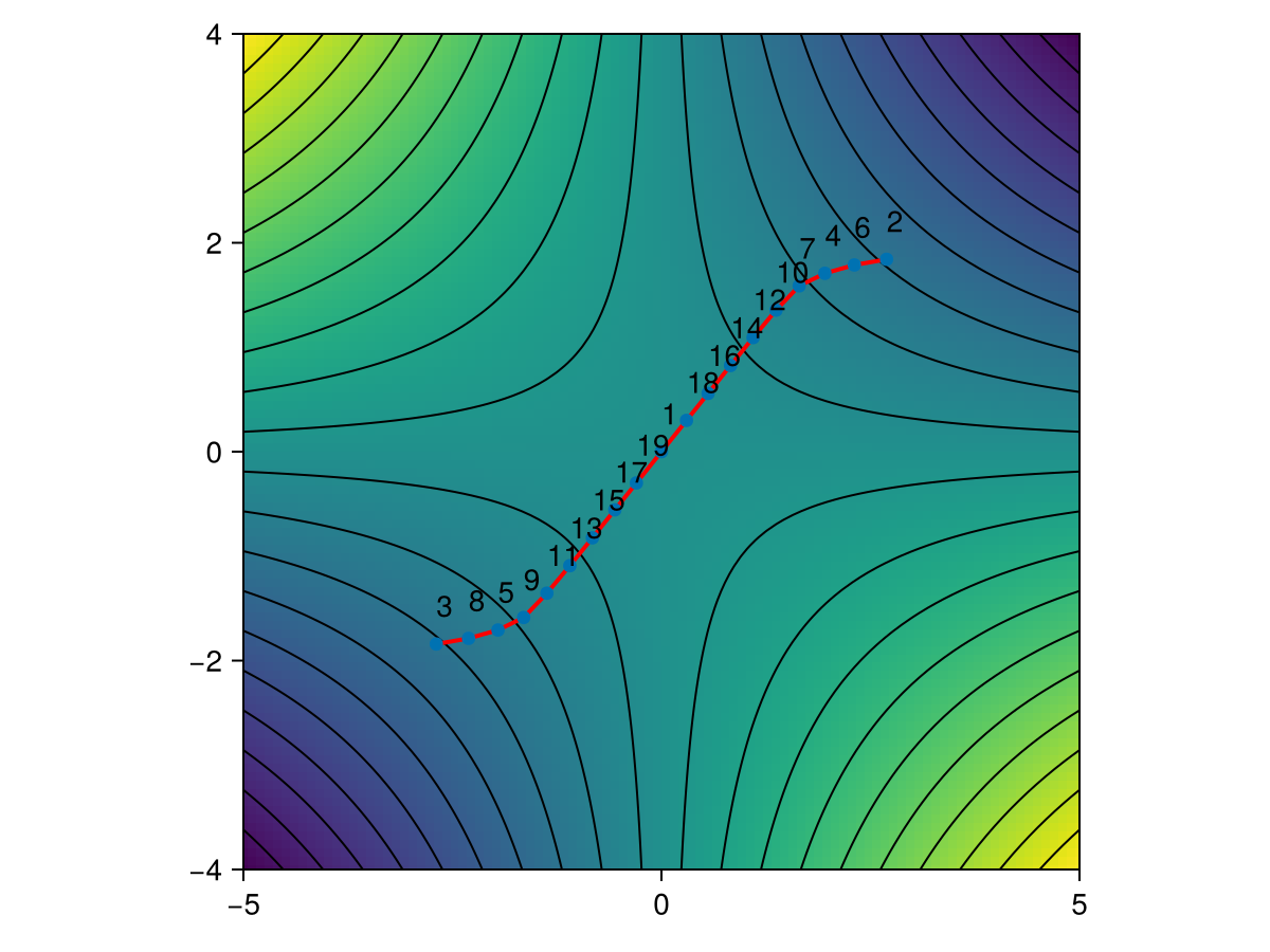
The integral evaluates to $(1+i)\sqrt{\pi/2}$
PL_integrate(S, thim, pars)1.2533126304104458 + 1.2533285739627602imPearcey integral
The Pearcey integral
\[I = \int_{-\infty}^\infty e^{i \omega(t^4 + x_2 t^2 + x_1 t)}\mathrm{d}t\]
is the canonical diffraction integral associated with the unfolding of the cusp catastrophe. We evaluate the thimbles on a coarse lattice in $x_1$ and $x_2$
using PicardLefschetzIntegration, ProgressMeter, Base.Threads, CairoMakie

pars = parameters(δ = 0.5, τ = -10., ϵ = 0.1, N = 50, n = 5, dim = 1)

S(p, x₁, x₂, ω) = ω * (p[1]^4 + x₂ * p[1]^2 + x₁ * p[1])

aRange_L, bRange_L = range(-2., 2., 8), range(-2., 2., 8)

thimbles = Array{thimble}(undef, length(aRange_L), length(bRange_L));
let ω = 1
    @showprogress Threads.@threads for (i, j) in collect(Iterators.product(eachindex(aRange_L),eachindex(bRange_L)))
        x₁, x₂ = aRange_L[i], bRange_L[j]

        thim = initialGrid([-4], [4], pars)
        flow!(p -> S(p, x₁, x₂, ω), thim, pars)
        thimbles[i, j] = thim
    end
end

map(t->length(t.simplices), thimbles)
8×8 Matrix{Int64}:
16 13 13 13 16 13 15 9
23 14 15 13 14 15 10 9
22 21 16 15 16 16 10 9
23 23 25 14 17 8 8 8
23 23 25 14 17 8 8 8
22 21 16 15 16 16 10 9
23 14 15 13 14 15 10 9
16 13 13 13 16 13 15 9Next, we evaluate the integral on a fine lattice in $x_1$ and $x_2$. Each thimble is converted once into a quadrature, which stores the quadrature nodes and weights, so that the many integrals reusing the same thimble are cheap.
quads = map(t -> quadrature(t, pars), thimbles)
aRange, bRange = range(-2., 2., 200), range(-2., 2., 200)

let ω = 20.
    data = zeros(Complex, length(aRange), length(bRange))

    @showprogress Threads.@threads for (i, j) in collect(Iterators.product(eachindex(aRange),eachindex(bRange)))
        x₁, x₂ = aRange[i], bRange[j]
        ii, jj = find_closest(aRange_L, x₁), find_closest(bRange_L, x₂)

        data[i, j] = PL_integrate(p -> S(p, x₁, x₂, ω), quads[ii, jj], pars)
    end

    fig = Figure()
    ax = Axis(fig[1, 1], aspect = 1)
    heatmap!(ax, aRange, bRange, abs.(data).^2, interpolate=true)
    fig
end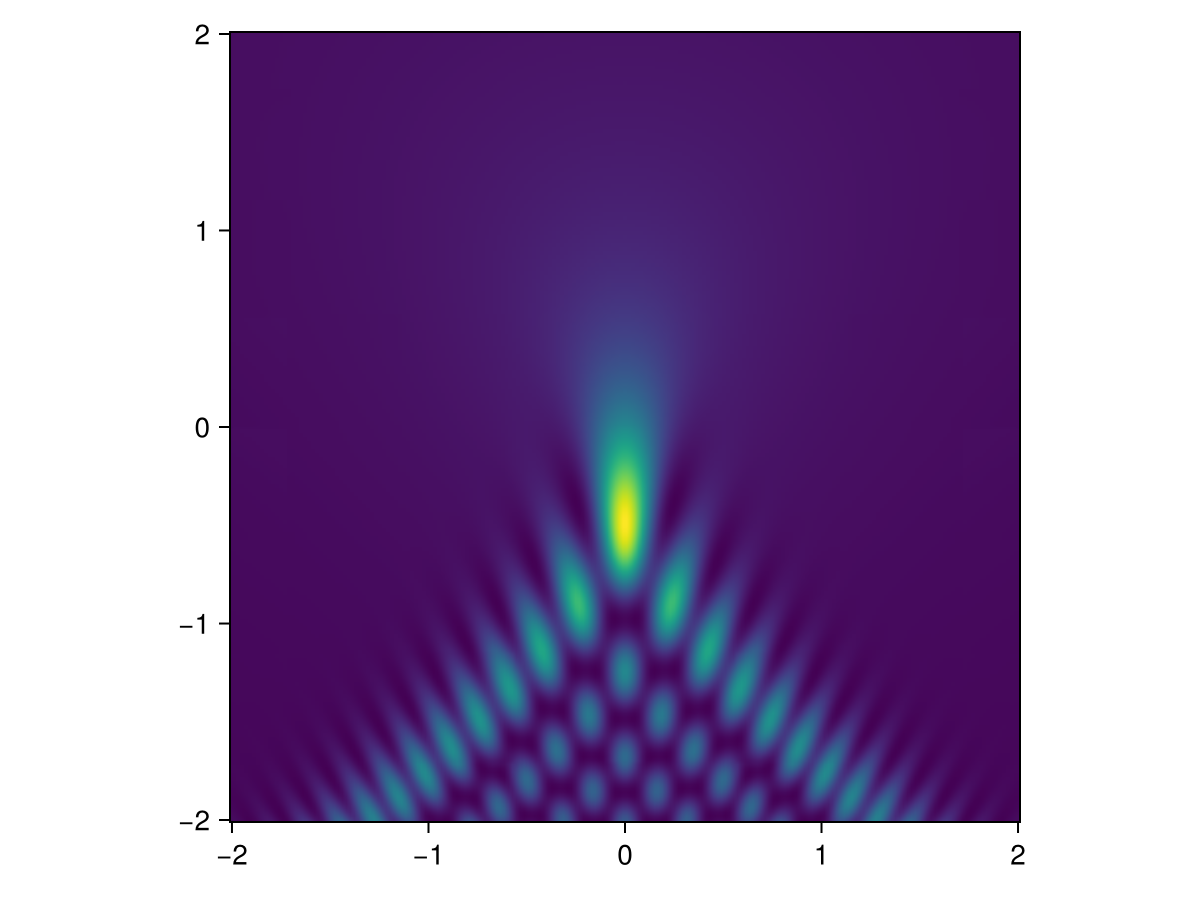
Elliptic integral
Consider the canonical diffraction integral associated with the unfolding of the elliptic integral
\[I = \int_{-\infty}^\infty \int_{-\infty}^\infty e^{i \omega \left( t^3 - 3 t v^2 - x_3 (t^2 + v^2) - x_2 v - x_1 t \right)}\mathrm{d}t \mathrm{d}v\,.\]
We evaluate the thimbles on a coarse lattice in $x_1$ and $x_2$ for $x_3 = 1$
using PicardLefschetzIntegration, ProgressMeter, Base.Threads, CairoMakie

pars = parameters(δ = 0.5, τ = -10., ϵ = 0.1, N = 20, n = 5, dim = 2)

S(p, x₁, x₂, x₃, ω) = ω * (p[1]^3 - 3. * p[1] * p[2]^2 - x₃ * (p[1]^2 + p[2]^2) - x₂ * p[2] - x₁ * p[1])

aRange_L, bRange_L = range(-2., 2., 8), range(-2., 2., 8)

thimbles = Array{thimble}(undef, length(aRange_L), length(bRange_L));
let ω = 1, x₃ = 1
    @showprogress Threads.@threads for (i, j) in collect(Iterators.product(eachindex(aRange_L),eachindex(bRange_L)))
        x₁, x₂ = aRange_L[i], bRange_L[j]

        thim = initialGrid([-4, -4], [4, 4], pars)
        flow!(p -> S(p, x₁, x₂, x₃, ω), thim, pars)
        thimbles[i, j] = thim
    end
end

map(t->length(t.simplices), thimbles)
8×8 Matrix{Int64}:
862 1017 1197 1131 1131 1197 1017 862
869 1171 1245 1331 1331 1245 1171 869
954 977 1083 1530 1530 1083 977 954
1117 1226 1353 1662 1662 1353 1226 1117
1136 1224 1390 1538 1538 1390 1224 1136
1166 1224 1309 1459 1459 1309 1224 1166
1130 1191 1167 1132 1132 1167 1191 1130
1043 1122 998 927 927 998 1122 1043Next, we evaluate the integral on a fine lattice in $x_1$ and $x_2$. Each thimble is converted once into a quadrature, which stores the quadrature nodes and weights, so that the many integrals reusing the same thimble are cheap.
quads = map(t -> quadrature(t, pars), thimbles)
aRange, bRange = range(-2., 2., 100), range(-2., 2., 100)

let ω = 20, x₃ = 1
    data = zeros(Complex, length(aRange), length(bRange))

    @showprogress Threads.@threads for (i, j) in collect(Iterators.product(eachindex(aRange),eachindex(bRange)))
        x₁, x₂ = aRange[i], bRange[j]
        ii, jj = find_closest(aRange_L, x₁), find_closest(bRange_L, x₂)

        data[i, j] = PL_integrate(p -> S(p, x₁, x₂, x₃, ω), quads[ii, jj], pars)
    end

    fig = Figure()
    ax = Axis(fig[1, 1], aspect = 1)
    heatmap!(ax, aRange, bRange, abs.(data).^2, interpolate=true)
    fig
end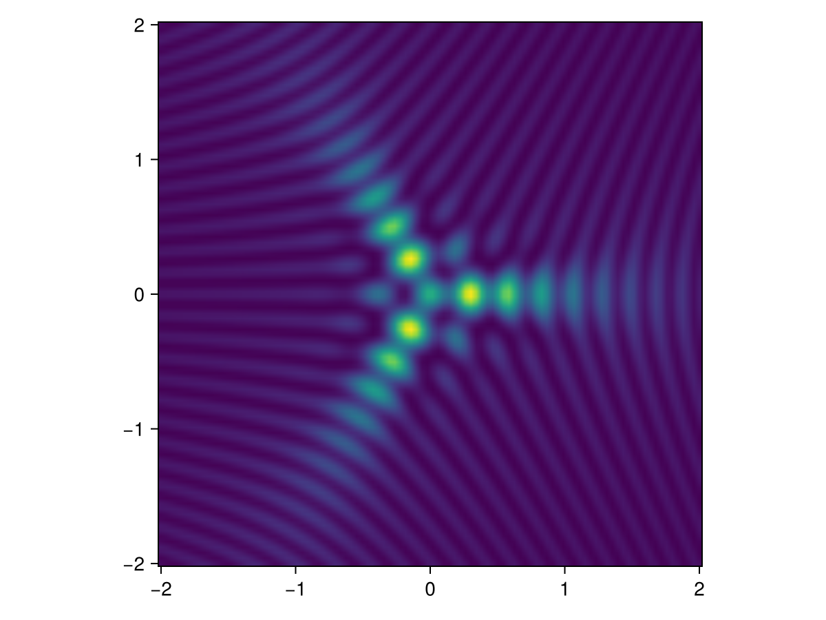
2D Gaussian lens
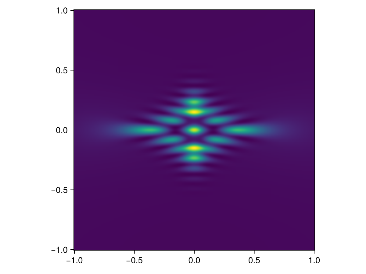
Consider the Kirchhoff-Fresnel diffraction integral associated with a thin Gaussian lens
\[I = \frac{\omega}{2\pi i} \int_{-\infty}^\infty \int_{-\infty}^\infty e^{i \omega \left( \frac{(\bm{x}-\bm{y})^2}{2} + e^{\frac{1+x_1^2 + 2 x_2^2}{2}} \right)}\mathrm{d}x_1 \mathrm{d}x_2\,.\]
We evaluate the thimbles on a coarse lattice in $y_1$ and $y_2$,
using PicardLefschetzIntegration, ProgressMeter, Base.Threads, CairoMakie, GeometryBasics

pars = parameters(δ = 1., τ = -10., ϵ = 0.1, N = 20, n = 8, dim = 2)

φ(p) = exp(- (p[1]^2 + 2 * p[2]^2) / 2)
T(p, y₁, y₂, ω) = ω * (((p[1] - y₁)^2 + (p[2] - y₂)^2) / 2. + φ(p))

aRange_L, bRange_L = range(-2., 2., 20), range(-2., 2., 20)

thimbles = Array{thimble}(undef, length(aRange_L), length(bRange_L));
let ω = 1
    @showprogress Threads.@threads for (i, j) in collect(Iterators.product(eachindex(aRange_L),eachindex(bRange_L)))
        y₁, y₂ = aRange_L[i], bRange_L[j]

        thim = initialGrid([-4, -4], [4, 4], pars)
        flow!(p -> T(p, y₁, y₂, ω), thim, pars)
        thimbles[i, j] = thim
    end
end

map(t->length(t.simplices), thimbles)
20×20 Matrix{Int64}:
540 566 594 617 636 637 649 673 … 649 637 636 617 594 566 540
566 596 622 642 676 648 684 702 684 648 676 642 622 596 566
577 612 641 643 672 673 690 711 690 673 672 643 641 612 577
604 619 646 680 707 710 729 732 729 710 707 680 646 619 604
621 648 658 686 732 754 777 754 777 754 732 686 658 648 621
630 663 673 703 711 741 752 772 … 752 741 711 703 673 663 630
646 706 714 752 748 731 755 768 755 731 748 752 714 706 646
632 697 696 749 753 738 757 750 757 738 753 749 696 697 632
670 727 718 732 760 771 776 763 776 771 760 732 718 727 670
650 729 750 741 770 772 787 756 787 772 770 741 750 729 650
650 729 750 741 770 772 787 756 … 787 772 770 741 750 729 650
670 727 718 732 760 771 776 763 776 771 760 732 718 727 670
632 697 696 749 753 738 757 750 757 738 753 749 696 697 632
646 706 714 752 748 731 755 768 755 731 748 752 714 706 646
630 663 673 703 711 741 752 772 752 741 711 703 673 663 630
621 648 658 686 732 754 777 754 … 777 754 732 686 658 648 621
604 619 646 680 707 710 729 732 729 710 707 680 646 619 604
577 612 641 643 672 673 690 711 690 673 672 643 641 612 577
566 596 622 642 676 648 684 702 684 648 676 642 622 596 566
540 566 594 617 636 637 649 673 649 637 636 617 594 566 540The thimbles look like
function plotMesh(thim::thimble)
    verts1 = map(p -> Point3f(real(p.coord[1]), real(p.coord[2]), imag(p.coord[1])), filter(p -> p.active, thim.points))
    verts2 = map(p -> Point3f(real(p.coord[1]), real(p.coord[2]), imag(p.coord[2])), filter(p -> p.active, thim.points))
    faces = map(p ->TriangleFace(p.coord), thim.simplices)

    fig = Figure()
    ax1 = Axis3(fig[1, 1], aspect = :data, xlabel = "Re[p₁]", ylabel = "Re[p₂]", zlabel = "Im[p₁]")
    ax2 = Axis3(fig[1, 2], aspect = :data, xlabel = "Re[p₁]", ylabel = "Re[p₂]", zlabel = "Im[p₂]")
    mesh!(ax1, verts1, faces, color = :orange, shading = true)
    mesh!(ax2, verts2, faces, color = :orange, shading = true)

    fig
end

plotMesh(thimbles[4, 4])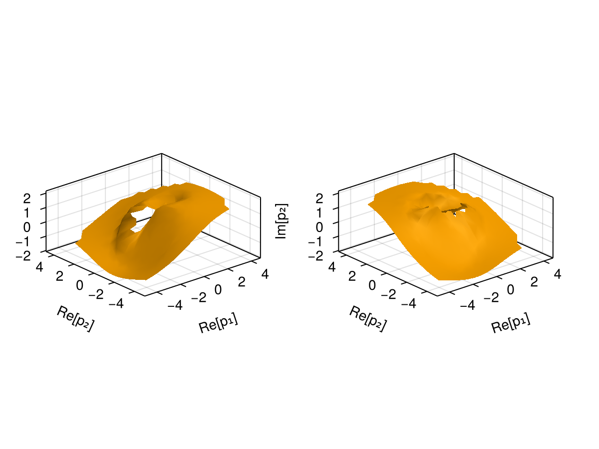
Next, we evaluate the integral on a fine lattice in $y_1$ and $y_2$. Each thimble is converted once into a quadrature, which stores the quadrature nodes and weights, so that the many integrals reusing the same thimble are cheap.
quads = map(t -> quadrature(t, pars), thimbles)
aRange, bRange = range(-1., 1., 200), range(-1., 1., 200);
let ω = 50
    data = zeros(Complex, length(aRange), length(bRange));
    Threads.@threads for (i, j) in collect(Iterators.product(eachindex(aRange),eachindex(bRange)))
        y₁, y₂ = aRange[i], bRange[j]
        ii, jj = find_closest(aRange_L, y₁), find_closest(bRange_L, y₂)

        data[i, j] = PL_integrate(p -> T(p, y₁, y₂, ω), quads[ii, jj], pars)
    end
    data = ω / (2π * im) .* data

    fig = Figure()
    ax = Axis(fig[1, 1], aspect = 1)
    heatmap!(ax, aRange, bRange, abs.(data).^2, interpolate=true)
    fig
end