Theory

Picard-Lefschetz theory formalises the famous saddle point method for multidimensional integrals. In the process, it provides a systematic method to evaluate highly oscillatory integrals. We here briefly describe Picard-Lefschetz theory and the implementation of the present package.

Picard-Lefschetz theory

For a $d$-dimensional oscillatory integral

\[I = \int_D e^{i k f(\boldsymbol{x})}\mathrm{d}\boldsymbol{x}\,,\]

with a meromorphic exponent $f$, we use Cauchy's integral theorem to deform the original integration domain into a set of steepest descent manifolds $\mathcal{J}_j$ in the complex plane $\mathbb{C}^d$,

\[I = \sum_j n_j \int_{\mathcal{J}_j} e^{i k f(\boldsymbol{x})}\mathrm{d}\boldsymbol{x}\,.\]

A saddle point is relevant, i.e, the descent manifold $\mathcal{J}_j$ associated with the critical point $\boldsymbol{x}_j$ contributes to the deformation when the intersection number $n_j \in \mathbb{Z}$ is non-zero. When $n_j \neq 0$, the critical point $\boldsymbol{x}_j$ is relevant to the integral. When $n_j=0$, the critical point $\boldsymbol{x}_j$ is irrelevant. Remarkably, the intersection number $n_j$ of the critical point $\boldsymbol{x}_j$ is given by the number of times its associated steepest ascent manifold $\mathcal{K}_j$ intersects the original integration domain $D$, i.e., $n_j = \langle D, \mathcal{K}_j\rangle$. This deformation is optimal as the Cauchy-Riemann equations guarantee that the integrand no longer oscillates along the steepest descent manifold.

Given an oscillatory integral, its evaluation has been reduced to computing the intersection numbers $n_j$ and the associated relevant steepest descent manifolds $\mathcal{J}_j$.

Integrating along the Lefschetz thimbles

The evaluation of the integral along the Lefschetz thimbles in the complex plane is implemented in five steps

This package triangulates the original integration domain $D$ into a set of simplices

\[\{[\boldsymbol{p}_{n_1}\dots \boldsymbol{p}_{n_{d+1}}], [\boldsymbol{p}_{n_{d+2}} \dots \boldsymbol{p}_{n_{2d+2}}], \dots \}\,.\]

We flow the vertices of the simplices in the complex plane, following the downward flow

\[\frac{\partial \gamma_\lambda(\boldsymbol{x}_0)}{\partial \lambda} = - \overline{\frac{\partial f(\gamma_\lambda(\boldsymbol{x}_0))}{\partial \boldsymbol{x}}}\,,\]

with the boundary condition $\gamma_{\lambda = 0}(\boldsymbol{x}_0) = \boldsymbol{x}_0$. In particular, using the Euler method, we evolve the points $\boldsymbol{p}_j$ using the rule

\[\boldsymbol{p}_j \mapsto \boldsymbol{p}_j - \epsilon \overline{\frac{\partial f(\boldsymbol{p}_j)}{\partial \boldsymbol{x}}}\,,\]

with step size $\epsilon$.

The downward flow of the original integration domain only converges to the relevant Lefschetz thimbles as a manifold, not as a set of points. Consequently, we need to subdivide the simplices when they become too large. Specifically, we check whether the longest edge of a simplex exceeds the threshold $\delta$ and split the simplex into two simplices by introducing a new vertex at the midpoint of the longest edge.
Finally, points for which the real part of the exponent

\[h(\boldsymbol{x}) = \text{Re}[i f(\boldsymbol{x})]\]

drops below the threshold $\tau$, can be safely removed from the tessellation of the integration domain as the integrand in the point and the consequent contribution to the integral becomes exponentially small.

Finally, after deforming the integration domain in the complex plane and approximating the relevant steepest descent manifolds, we integrate along the simplices with a simplex Gaussian quadrature scheme.

Example integral

We illustrate this integration scheme for the one-dimensional lens integral

\[\Psi(y) = \sqrt{\frac{\omega}{2\pi i}} \int_{-\infty}^\infty e^{i \omega \left(\frac{(x-y)^2}{2} + \frac{1}{1+x^2}\right)}\mathrm{d}x\,,\]

known as the one-dimensional Lorentzian lens model. This integral depends on the frequency $\omega$ and the time delay function

\[T(x,y) = \frac{(x-y)^2}{2} + \frac{1}{1+x^2}\,,\]

where the first term has a geometric origin, corresponding to the relative path length from the source to the point $x$ on the lens plane and the observer at $y$ in the image plane. The second term is the phase variation of the lens model.

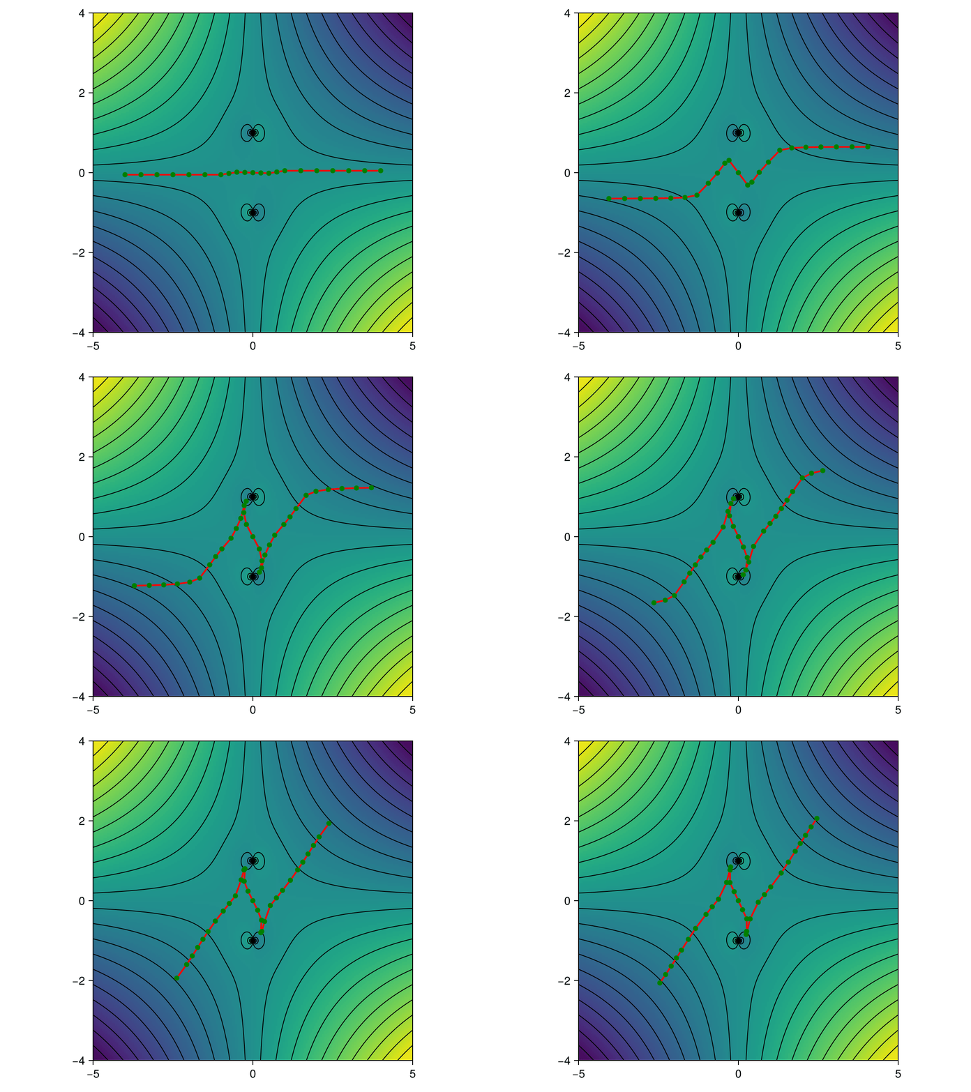
First, we represent the integration domain by a set of line segments. Next, we flow the line segments into the complex plane $\mathbb{C}$ using the downward flow. The flow converges to the relevant thimbles. For example, for $y=0$, we obtain the thimble

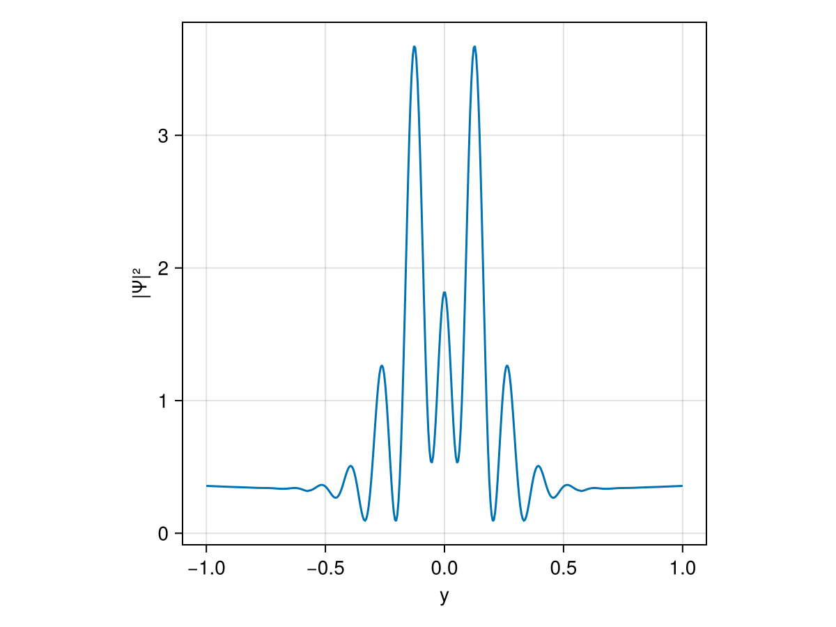
Along the deformed integration domain, the integrand no longer oscillates, allowing for an efficient evolution of the lens amplitude. The intensity $|\Psi(y)|^2$, with the angular frequency $\omega = 20$, assumes the form