Gravitational lensing

Gravitational lensing in the thin-lens approximation, where the region over which the radiation is significantly deflected is small compared to the distance the radiation travels from the source to the lens and from the lens to the observer, can be expressed in terms of the two-dimensional Kirchhoff-Fresnel integral

\[\psi(\boldsymbol{\mu}) = \frac{\nu}{2\pi i} \int e^{i \nu \left[(\boldsymbol{x}-\boldsymbol{\mu})^2/2 + \varphi(\boldsymbol{x})\right]} \mathrm{d}\boldsymbol{x}\]

with the position on the sky \(\boldsymbol{\mu}\), the position on the lens plane \(\boldsymbol{x}\), and the frequency of the radiation \(\nu\) in units of the Einstein radius. For the gravitational lensing by \(N\) point-sources positioned at \(\boldsymbol{x}_i\) the phase variation \(\varphi\) of the form

\[\varphi(\boldsymbol{x}) =- \sum_{i=1}^N f_i \log(\|\boldsymbol{x} - \boldsymbol{x}_i\|),\]

with \(f_i\) the relative strength of the lenses (determined by the masses of the sources), with \(f_1+\dots + f_N=1\). The intensity is defined as the magnitude squared of the amplitude

\[I(\boldsymbol{\mu}) = | \psi(\boldsymbol{\mu})|^2.\]

When the frequency is small compared to the Einstein radius, or when the radiation is incoherent, the geometric optics limit is a good approximation to this integral. However, when these conditions are not fulfilled we need to evaluate the highly oscillatory Kirchhoff-Fresnel integral to model the interference pattern. We will here describe the evaluation of the integral with Picard-Lefschetz theory.

Single gravitational lens

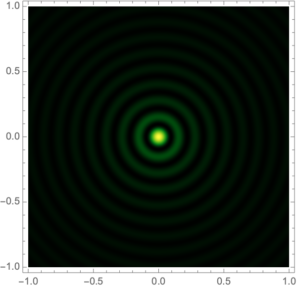
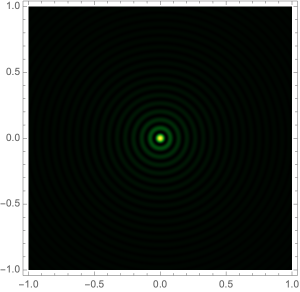
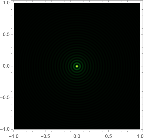
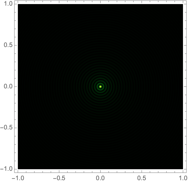
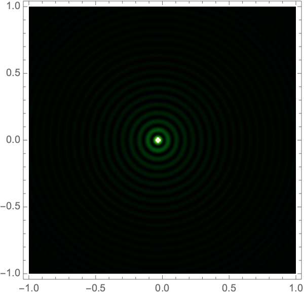
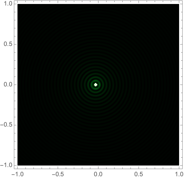
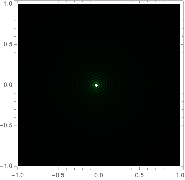
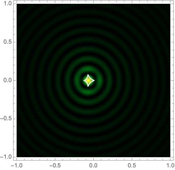
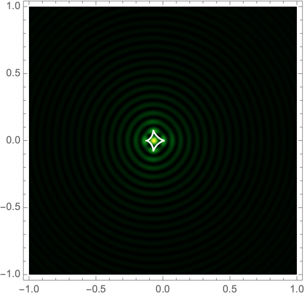
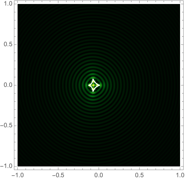
Lensing by a single point source, i.e., \(\varphi(\boldsymbol{x}) = -\log(\|x\|)\), is one of the few lensing integrals with a closed form solution

\[I(\boldsymbol{\mu}) = \frac{\pi \nu}{1-e^{-\pi \nu}} |_1F_1(i \nu / 2, 1; i \nu \mu^2/2)|^2,\]

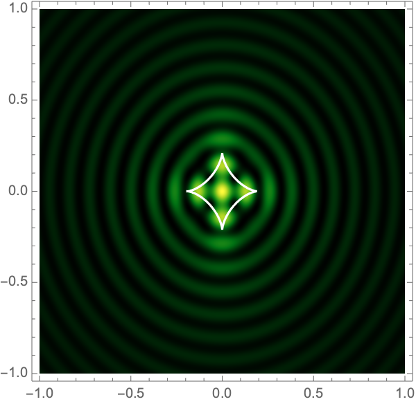
with \(\mu = \|\boldsymbol{\mu}\|\). See Fig. 1 for the interference patterns of the single gravitational lens.

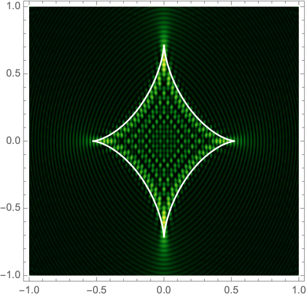
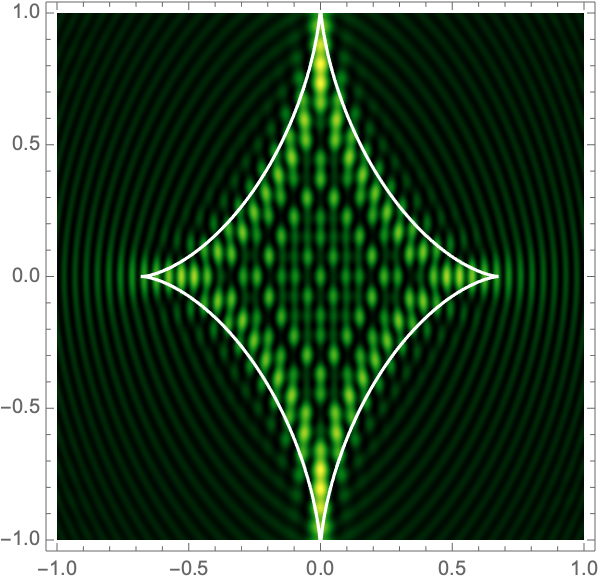
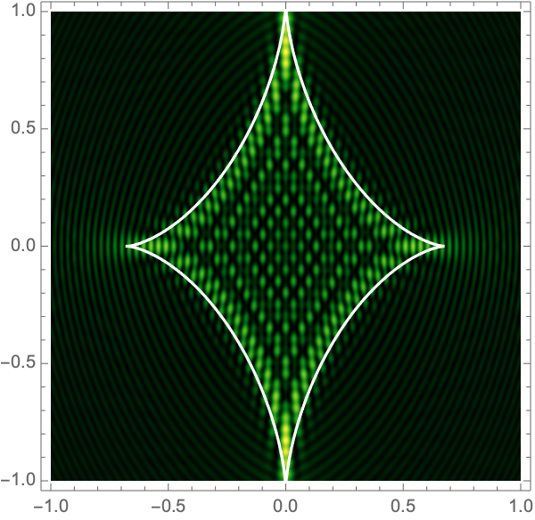
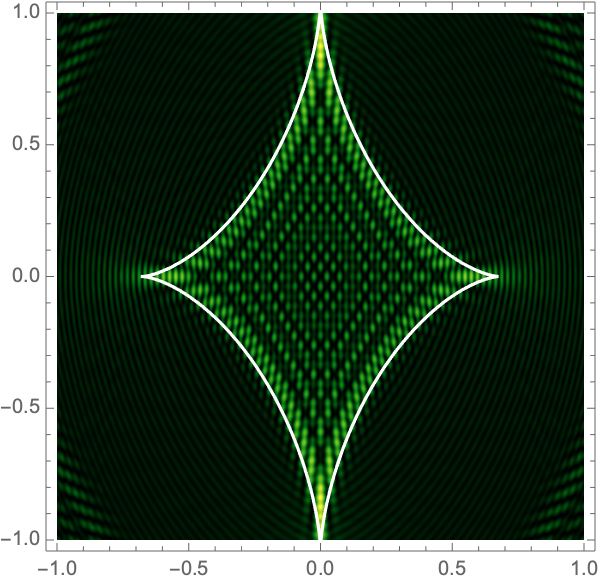
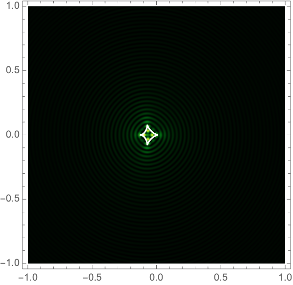
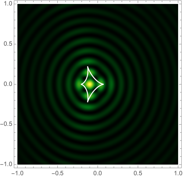
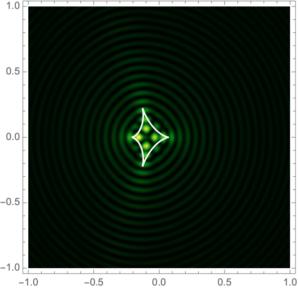
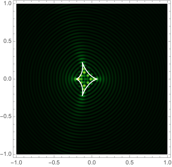
This is a beautiful result, but is unfortunately degenerate as a small perturbation of the phase variation will induce a dramatic change in the structure of the caustics and the interference pattern. More realistic is the occurrence of the single gravitational lens with a shear field,

\[\varphi(\boldsymbol{x}) = - \log(\|\boldsymbol{x}\|) + \frac{1}{2}\gamma (x^2 - y^2),\]

with \(\boldsymbol{x}=(x,y)\) and the strength of the shear \(0\leq \gamma \leq 1\). The additional term could, for example, represent the tidal force form an external mass located a distance \(\gamma^{-1/2}\) from the lens. In geometric optics, the single lens with a shear field induces the Lagrangian map,

\[\xi(\boldsymbol{x}) = \left(1-\frac{1}{\|\boldsymbol{x}\|}\right) \boldsymbol{x} +\gamma (-x,y),\]

sending points from the lens-plane to the screen. This map forms a caustic at the critical curve defined by the condition \(\det(\nabla \xi) = 0\),

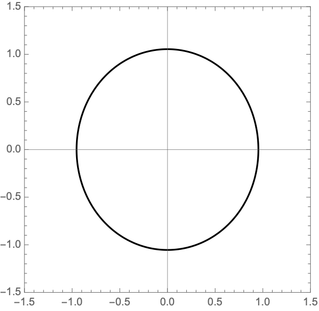
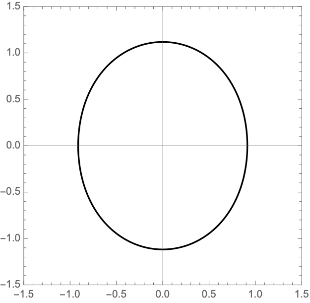
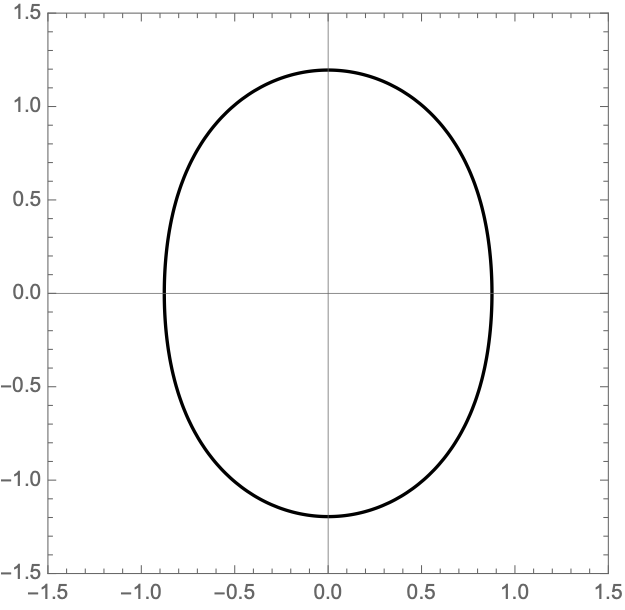
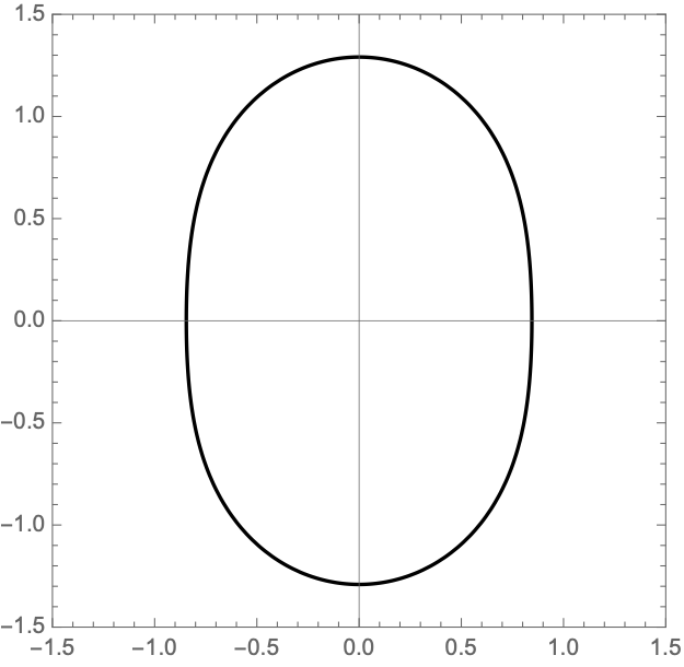
\[\mathcal{M} =\left \{ r (\cos \theta, \sin \theta) \,\bigg| \,r = \frac{1}{\sqrt{1- \gamma^2}} \sqrt{ \sqrt{1-\gamma^2 \sin^2 2 \theta} -\gamma \cos 2 \theta} \text{ and } \theta \in [0,2\pi)\right\}.\]

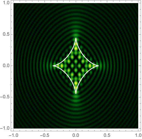
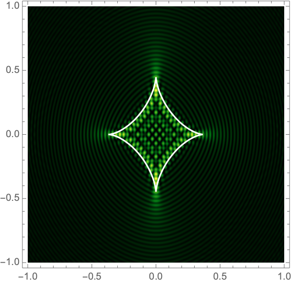
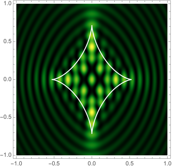
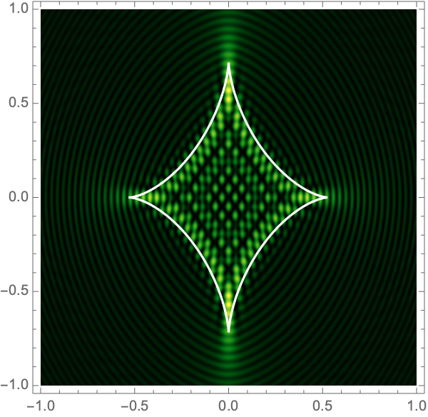
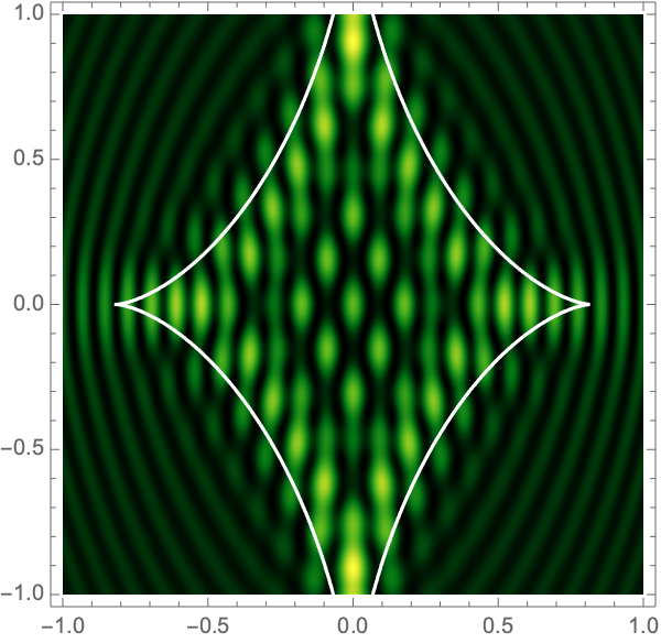
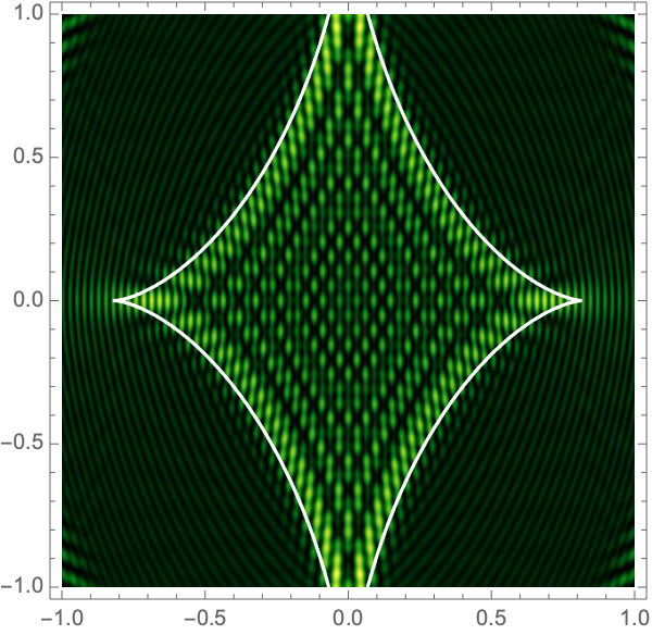
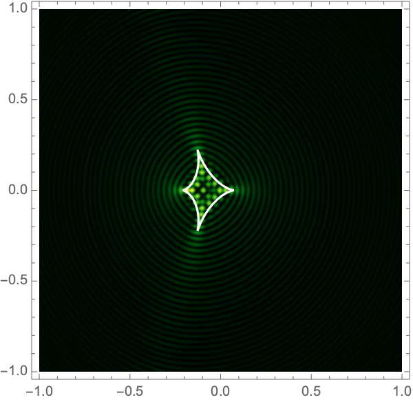
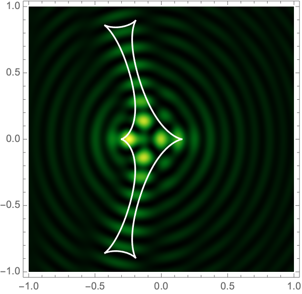
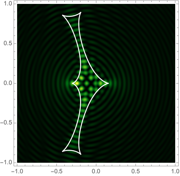
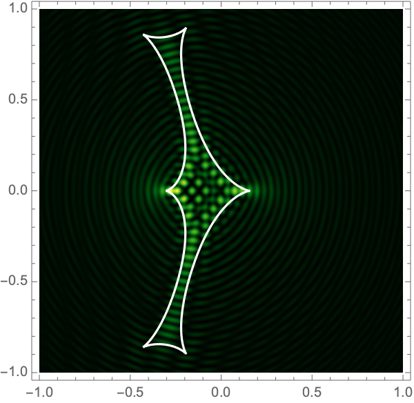
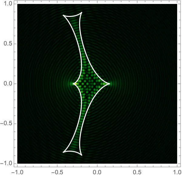
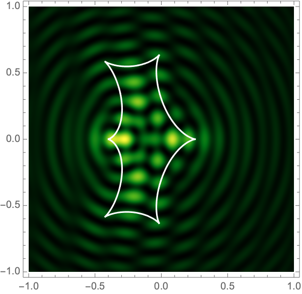
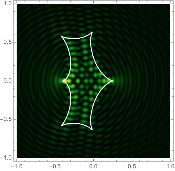
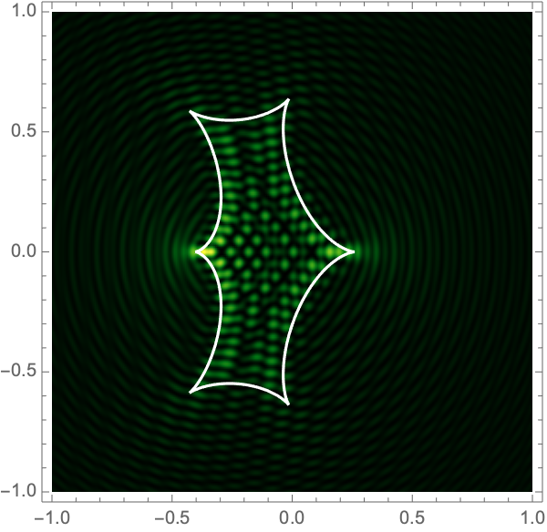
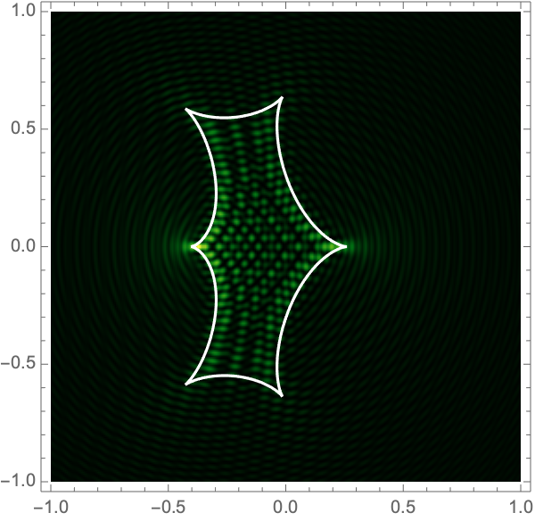
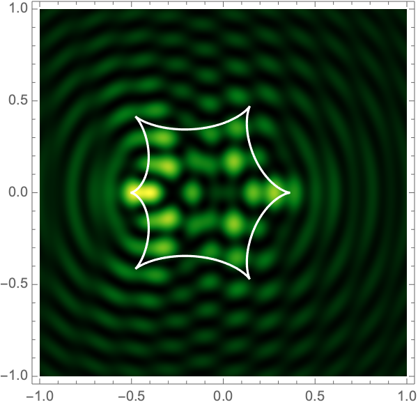
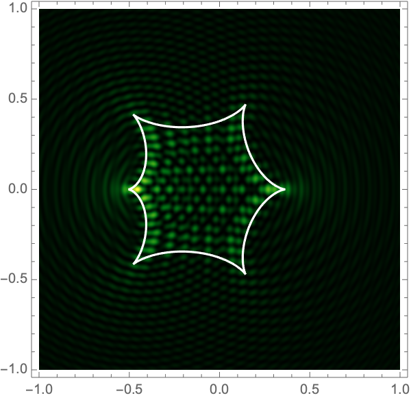
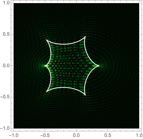
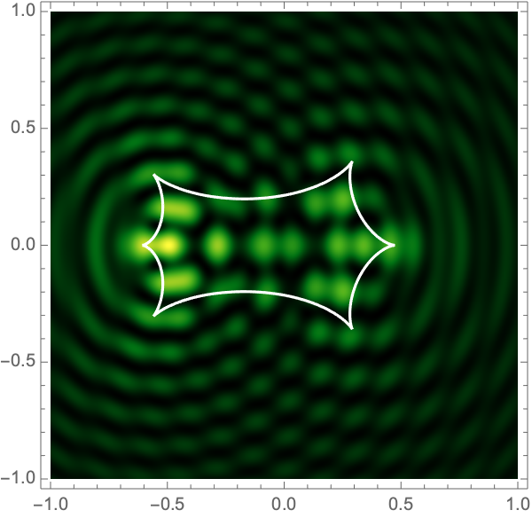
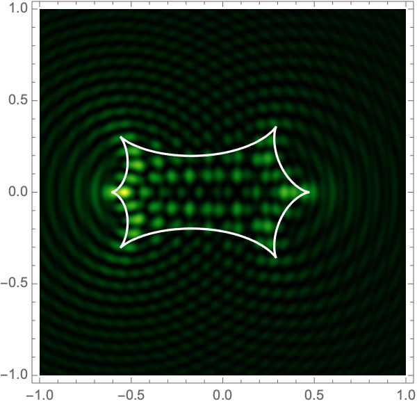
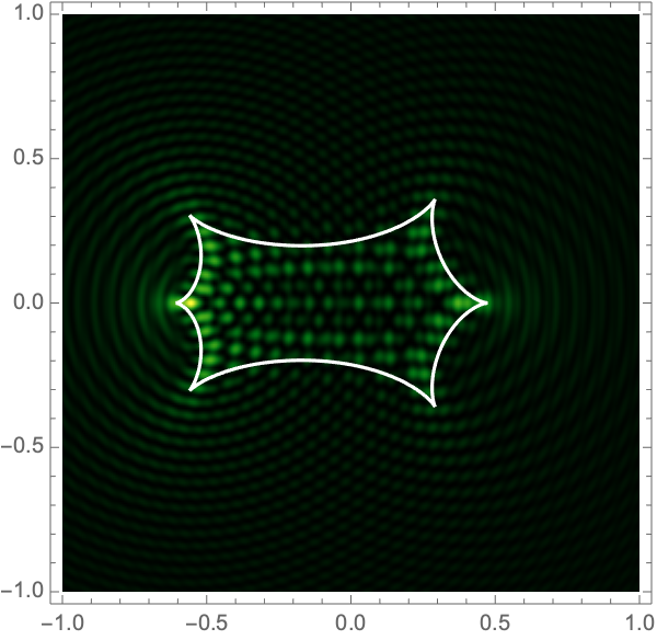
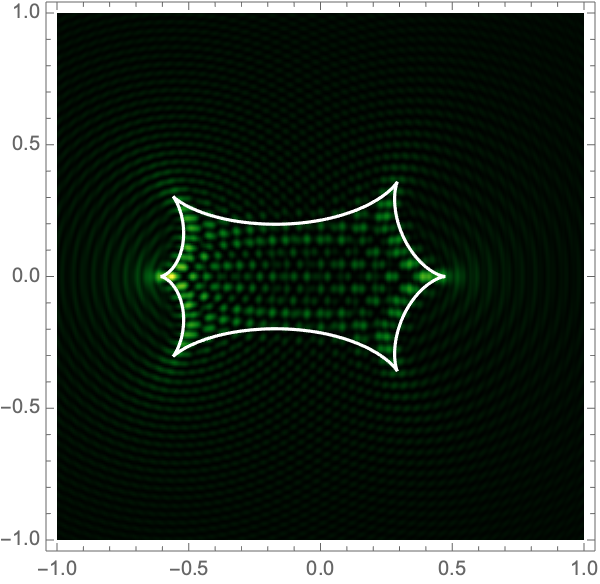
The Lagrangian map maps the critical curve to the caustic curve \(\xi(\mathcal{M})\) consisting of four fold curves running between four cusp points forming a curved diamond. This diamond is the curve at which the intensity in the geometric optics approximation diverges. The Kirchhoff-Fresnel integral has generically four saddle points, with two or four being real depending on whether \(\boldsymbol{\mu}\) is outside or inside the caustic curve. The outside and inside of the caustic curve are respectively double- and quadruple-image regions.

To evaluate the lens in wave optics, we use polar coordinates centered at the lens \(\boldsymbol{x} = r(\cos \theta , \sin \theta )\). In these coordinates, the integrand is an analytic function of the radial and angular coordinates,

\[\psi(\boldsymbol{\mu}) =\frac{\nu}{2\pi i} \int_{0}^\infty \int_0^{2\pi} e^{i \nu \left[ ((r\cos \theta - \mu_x)^2 + (r\sin \theta - \mu_y)^2) / 2 - \log r + \frac{\gamma }{2} r^2(\cos^2\theta - \sin^2\theta) \right]} r \mathrm{d} \theta \mathrm{d} r,\]

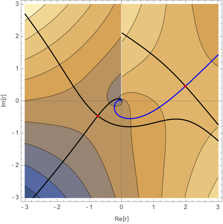
with \(\boldsymbol{\mu} = (\mu_x,\mu_y)\). As the angular integral is over a compact domain, we will use Picard-Lefschetz theory of the radial integral

\[g_{\theta}(\boldsymbol{\mu}) = \int_{\mathcal{J}_\theta} e^{i \nu \left[ ((r\cos \theta - \mu_x)^2 + (r\sin \theta - \mu_y)^2) / 2 - \log r + \frac{\gamma }{2} r^2(\cos^2\theta - \sin^2\theta) \right] + \log r} \mathrm{d} r,\]

with the Lefschetz-thimble \(\mathcal{J}_\theta\) the complex continuous deformation of the original integration domain \((0,\infty)\). This deformation is obtained using Picard-Lefschetz theory, removing the oscillations from the radial integral (see Fig. 3 for an example).

The remaining integral over the angular parameter

\[\psi(\boldsymbol{\mu}) =\frac{\nu}{2\pi i} \int_0^{2\pi} g_\theta (\boldsymbol{\mu})\mathrm{d}\theta,\]

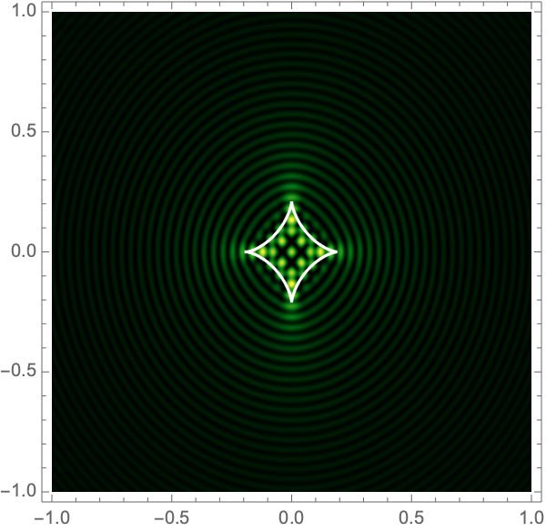
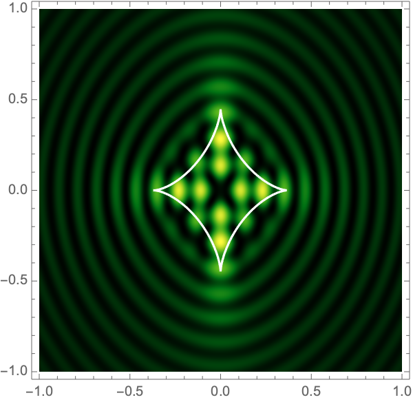
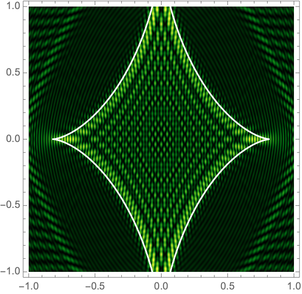
can be evaluated with traditional numerical methods. See Fig. 4 for the interference patterns of the single gravitational lens with a shear of \(\gamma=0.1,0.2,0.3, 0.4\) and \(0.5\) for the frequencies \(\nu=25,50,75,\) and \(100\).

Binary gravitational lens

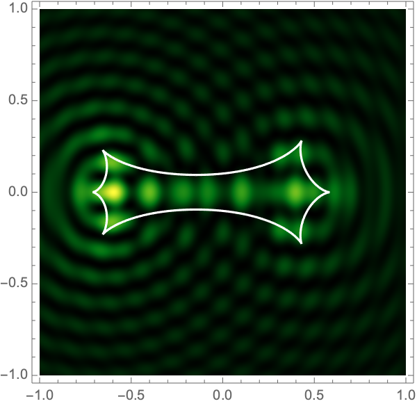
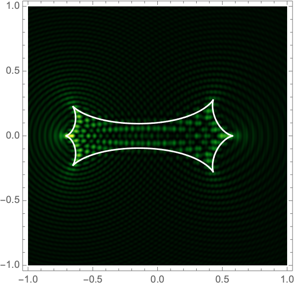
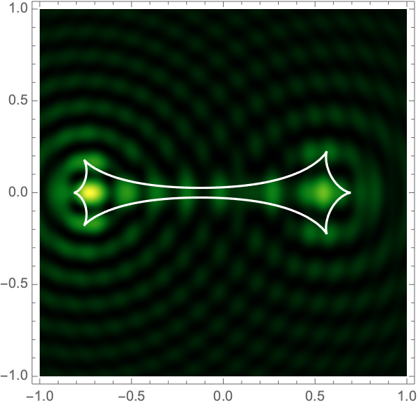
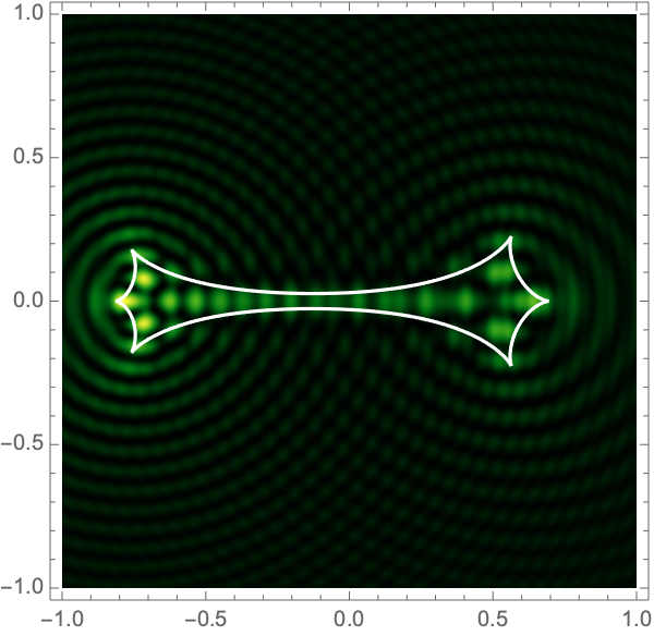
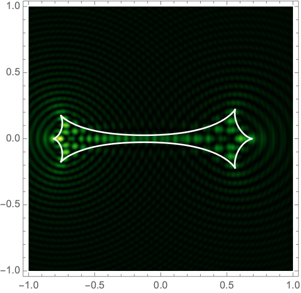
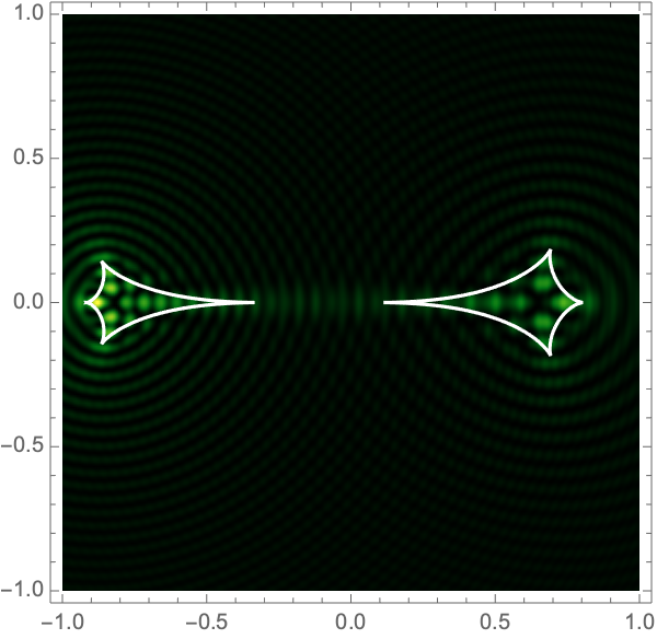
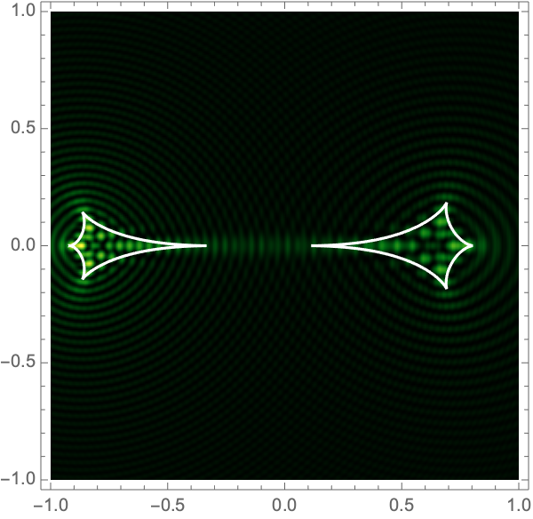
The binary gravitational lens is described by the phase variation

\[\varphi(\boldsymbol{x}) = -f_1 \log(\|\boldsymbol{x} - \boldsymbol{x}_1\|) - f_2 \log(\|\boldsymbol{x} - \boldsymbol{x}_2\|).\]

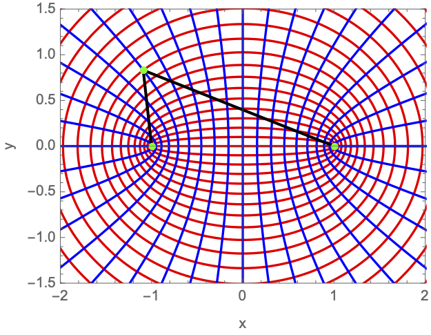
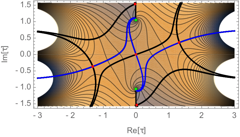
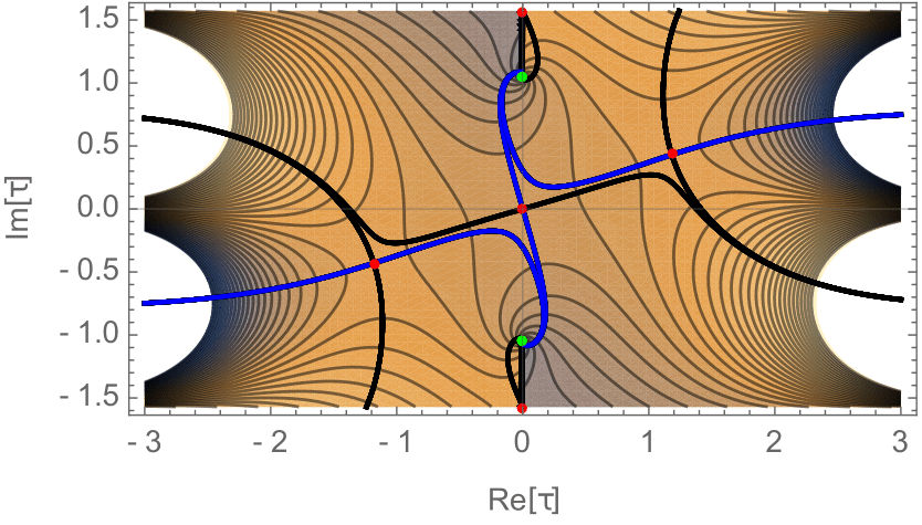
For simplicity, we will let \(\boldsymbol{x}_1 = (-a,0)\) and \(\boldsymbol{x}_1 = (a,0)\) for some \(a>0\). Using elliptic coordinates, \(\boldsymbol{x}(\tau,\sigma) = a(\cosh \tau \cos \sigma, \sinh \tau \sin \sigma)\), with \(0 < \tau < \infty\) and \(0 < \sigma \leq 2\pi\). Geometrically, the elliptic coordinates has two foci at the locations of the binary \(\boldsymbol{x}_1\) and \(\boldsymbol{x}_2\). The constant \(\tau\) contours form ovals around the foci (the red curves in Fig. 5). The constant \(\sigma\) contours pass between the to foci (the blue curves in Fig. 5).

Note that the variables \(\tau\) and \(\sigma\) resemble the radial and angular polar variables \(r\) and \(\theta\). In elliptic coordinates, we obtain the identities

\[ \begin{aligned} \|\boldsymbol{x} - \boldsymbol{x}_1\| &= a(\cosh \tau + \cos \tau),\\ \|\boldsymbol{x} - \boldsymbol{x}_2\| &= a(\cosh \tau - \cos \tau). \end{aligned}\]

In the measure in Cartesian and elliptic coordinates are related by the Jacobian

\[J(\tau,\sigma) = \frac{a^2}{2} \left( \cosh 2\tau - \cos 2 \sigma\right).\]

Following the calculation for the single gravitational lens, we perform the radial \(\tau\)-integral using Picard-Lefschetz theory

\[g_\sigma(\boldsymbol{\mu}) = \int_{\mathcal{J}_\sigma} e^{i \nu \left[ \frac{1}{2}(\boldsymbol{x}(\tau,\sigma) - \boldsymbol{\mu})^2 - f_1 \log(a(\cosh \tau + \cos \tau))- f_2 \log(a(\cosh \tau - \cos \tau))\right] + \log(J(\tau,\sigma))}\mathrm{d}\tau.\]

For this integral, it turns out to be most efficient to extend the original integration domain for \(\tau\) to the real line \(\mathbb{R}\). See Fig. 6 for two examples of the thimble \(\mathcal{J}_\sigma\).

The amplitude is now expressed as an angular integral over a compact domain which we evaluate using conventional integration techniques

\[\psi(\boldsymbol{\mu}) = \frac{\nu}{4\pi i} \int_0^{2\pi} g_{\sigma}(\boldsymbol{\mu}) \mathrm{d}\sigma.\]

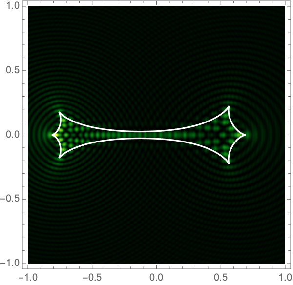
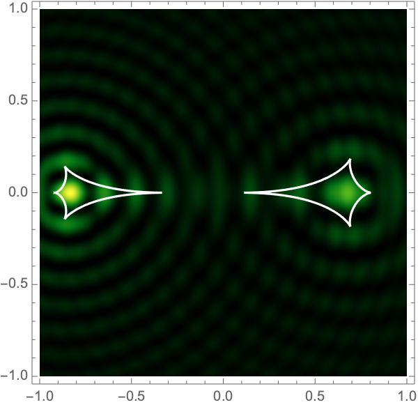
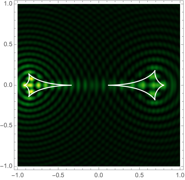
For an illustration of the intensity map for lens strenghts \(f_1=1/3, f_2=2/3\), with a seperation \(a=0.1,0.2,\dots,1.0\), and the frequencies \(\nu=25,50,75,\) and \(100\) see Fig. 7.