Tutorial
In this tutorial, we demonstrate the usage of the PhaseSpaceDTFE.jl package to estimate the density and velocity fields from a GADGET-4 simulation.
We start by importing the relevant libraries and loading the data:
using JLD2, Plots, HDF5, ProgressMeter, PhaseSpaceDTFE

## set up simulation box
Ni = 64
L  = 100.
sim_box = SimBox(L, Ni)   ## need this for estimator creation

depth   = 5   # depth of estimator search tree

## load data
function load_data(file)
    fid = h5open(file, "r")
    pos = convert.(Float64, read(fid["PartType1"]["Coordinates"]))
    vel = convert.(Float64, read(fid["PartType1"]["Velocities"]))
    ids = read(fid["PartType1"]["ParticleIDs"])
    time = read_attribute(fid["Header"], "Time")
    close(fid)

    ordering = sortperm(ids)
    return (copy(pos[:,ordering]'), copy(vel[:,ordering]'), time)
end

function load_mass(file)
    f = h5open(file, "r")
    read_attribute(f["Header"], "MassTable")[2]  # particle type 1
end

m = load_mass("../../test/data/snapshot_000.hdf5")
(coords_q, _, _) = load_data("../../test/data/snapshot_000.hdf5")
(coords_x, vels, _) = load_data("../../test/data/snapshot_002.hdf5")
([95.94856262207031 98.76901245117188 99.14542388916016; 99.86626434326172 97.77499389648438 97.80353546142578; … ; 94.38851928710938 97.52845764160156 0.3155221939086914; 94.68167114257812 97.48580169677734 99.97648620605469], [-292.1794128417969 -76.47138977050781 28.625730514526367; -60.02801513671875 -113.5673599243164 -126.30517578125; … ; -395.4625244140625 163.2576141357422 155.2444610595703; -418.26104736328125 123.40419006347656 328.3358459472656], 0.9999999999999997)The particle coordinates and velocities are Float64 matrices of size (N, 3). The particle mass m is a single Float64 or a vector of length N for individual particle masses.
Prequel: Delaunay Tesselation Field Estimator
Before going though through PS-DTFE method, we demonstrate the traditional DTFE method by calling the PS-DTFE code only on the final (Eulerian) particle positions. For details, see examples below.
## construct estimator
ps_dtfe = PS_DTFE_periodic(coords_x, coords_x, vels, m, depth, sim_box)
## This is equivalent to the DTFE_periodic routine
# ps_dtfe = DTFE_periodic(coords_x, vels, m, depth, sim_box)

## evaluate density field
Range = 0:0.2:100.
density_field = [PhaseSpaceDTFE.density([L/2., y, z], ps_dtfe) for y in Range, z in Range]
heatmap(Range, Range, log10.(density_field), aspect_ratio=:equal, xlims=(0, L), ylims=(0, L), c=:grays, xlabel="[Mpc]", ylabel="[Mpc]")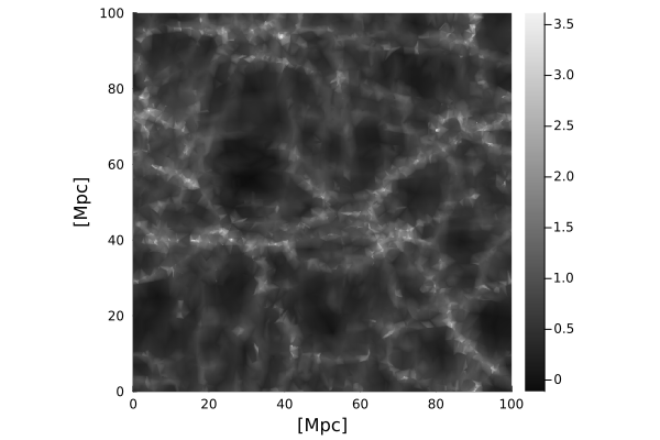
Phase-Space Delaunay Tessellation Field Estimator — basic implementation
We now demonstrate the use of the PS-DTFE method with the basic implementation that is suitable to simulations up to size 128^3 particles.
The first step is the construction of the estimator object from the initial (Lagrangian) and final (Eulerian) positions, coords_q and coords_x. This is done only once as a pre-computation step.
## construct estimator
ps_dtfe = PS_DTFE_periodic(coords_q, coords_x, vels, m, depth, sim_box)

## if want to ignore velocities
# ps_dtfe = PS_DTFE_periodic(coords_q, coords_x, m, depth, sim_box)

## for further use without pre-computation, consider saving the estimator to file
# save("ps_dtfe.jld2, "ps-dtfe", ps_dtfe)
nothing
The argument depth specifies the simplex search tree depth in the estimator. Higher tree depths result in faster field evaluations, but require longer construction times. We recommend to start with depth=5 and to increase this if required for high-resolution density fields.
The construction time should be of order 1-2 minutes for a 64^3 simulation at depth=7, or a 128^3 simulation at depth=5 on a modern computer.
We now evaluate the density field with the density()-function:
# evaluate density field
density_field = [PhaseSpaceDTFE.density([L/2., y, z], ps_dtfe) for y in Range, z in Range]
heatmap(Range, Range, log10.(density_field), aspect_ratio=:equal, xlims=(0, L), ylims=(0, L), c=:grays, xlabel="[Mpc]", ylabel="[Mpc]")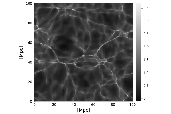
The corresponding number of streams is evaluated with the numberOfStreams()-function:
nstreams_field = [numberOfStreams([L/2., y, z], ps_dtfe) for y in Range, z in Range]
heatmap(Range, Range, nstreams_field, aspect_ratio=:equal, xlims=(0, L), ylims=(0, L), clim=(1, 7), xlabel="[Mpc]", ylabel="[Mpc]")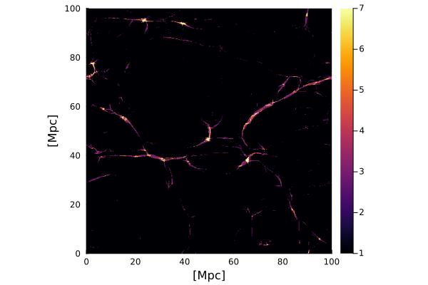
Similarly, the velocity field is evaluated with the velocity()-function:
velocity_field = [velocity([L/2., y, z], ps_dtfe) for y in Range, z in Range]501×501 Matrix{Matrix{Float64}}:
[20.7923 -68.3154 26.7559] … [20.1516 -93.5948 19.9205]
[20.0133 -66.183 24.3481] [19.3726 -91.4624 17.5128]
[19.2342 -64.0506 21.9404] [18.5935 -89.33 15.105]
[20.4166 -79.3451 20.7265] [29.5419 -77.6228 12.427]
[21.1161 -76.0055 18.2847] [30.2414 -74.2832 9.98515]
[21.8157 -72.6659 15.8428] … [30.941 -70.9436 7.54331]
[22.5152 -69.3264 13.401] [31.6405 -67.604 5.10146]
[23.2148 -65.9868 10.9591] [32.3401 -64.2645 2.65961]
[23.9143 -62.6472 8.5173] [33.0396 -60.9249 0.217766]
[24.6139 -59.3076 6.07545] [33.7392 -57.5853 -2.22408]
⋮ ⋱ ⋮
[45.407 -114.853 36.2093] [19.4907 -114.9 43.0973]
[42.7378 -111.405 34.8192] [16.8215 -111.451 41.7072]
[34.5435 -106.983 31.5999] [20.5576 -109.429 34.7492]
[31.9363 -103.453 30.0963] … [17.9504 -105.899 33.2457]
[29.3292 -99.9225 28.5927] [15.3433 -102.368 31.7421]
[44.4834 -111.786 23.9269] [22.7914 -92.7107 29.2348]
[43.6918 -109.956 21.4322] [21.9998 -90.8807 26.7402]
[20.9307 -95.7272 22.3283] [20.9307 -95.7272 22.3283]
[20.1516 -93.5948 19.9205] … [20.1516 -93.5948 19.9205]In multistream regions, the velocity()-function returns the velocities of the individual streams (or NaN if single_stream=true is set in the function). To obtain the stream-mass weighted summation of the velocities, call the velocitySum()-function, which reduces to the velocity()-function in single-stream regions.
velocity_field = [velocitySum([L/2., y, z], ps_dtfe) for y in Range, z in Range]For large simulations when aiming at evaluating the PS-DTFE field in a slice, it can be beneficial to first select the $N$-body particles lying near the slice (in a slab of thickness $\epsilon$) before constructing the estimator.
using Base.Threads

function density_slice(coords_q, coords_x, p, dim, ϵ, m, depth, box, range)
	println("Filter field")
	filter = p[dim] - ϵ .< coords_x[:, dim] .< p[dim] + ϵ

	coords_q_reduced = coords_q[filter, :]
	coords_x_reduced = coords_x[filter, :]

	println("Generate estimator")
	ps_dtfe = PS_DTFE_periodic(coords_q_reduced, coords_x_reduced, m, depth, box)

	dfield = zeros((length(range), length(range)))
	nfield = zeros((length(range), length(range)))

	println("Evalaute density field")
	@showprogress Threads.@threads for I in CartesianIndices(dfield)
    	i, j = Tuple(I)
		@inbounds x, y = range[i], range[j]

		P = [x, y]
		insert!(P, dim, p[dim])
		@inbounds dfield[i, j] = PhaseSpaceDTFE.density(P, ps_dtfe)
		@inbounds nfield[i, j] = PhaseSpaceDTFE.numberOfStreams(P, ps_dtfe)
	end

	return dfield, nfield
end

let dim = 1, ϵ = 2., depth = 7
    global dfield, nfield = density_slice(coords_q, coords_x, [L / 2., L / 2., L / 2.], dim, ϵ, m, depth, sim_box, Range)
end

heatmap(Range, Range, log10.(dfield), aspect_ratio=:equal, xlims=(0, L), ylims=(0, L), c=:grays, xlabel="[Mpc]", ylabel="[Mpc]")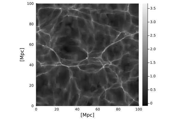
heatmap(Range, Range, nfield, aspect_ratio=:equal, xlims=(0, L), ylims=(0, L), clim=(1, 7), xlabel="[Mpc]", ylabel="[Mpc]")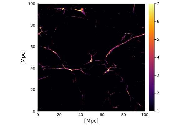
The Phase-Space Delaunay Tessellation Field Estimator — subbox implementation
We now demonstrate the use of the PS-DTFE method for simulations with more than 128^3 particles.
It is not feasible to directly apply the basic PS-DTFE implementation to high-resolution simulations, as the construction of the estimator's simplex search tree would require immense working memory (> 100 GB for 256^3 particles). To circumvent this, the subbox routine internally divides the simulation box into smaller subboxes, constructs an estimator for each of these and writes the subbox estimators to file. The user constructs the ps_dtfe_sb object holding the subbox references as follows:
## construct estimator with velocities
ps_dtfe_sb = ps_dtfe_subbox(coords_q, coords_x, vels, m, depth, sim_box; N_target=32)

## construct estimator without velocities
# ps_dtfe_sb = ps_dtfe_subbox(coords_q, coords_x, m, depth, sim_box; N_target=32)

## it is recommended to save the estimator object (holding the subbox references) for further use
save("ps_dtfe_sb.jld2", "ps-dtfe-sb", ps_dtfe_sb)
ps_dtfe_sb = load("ps_dtfe_sb.jld2")["ps-dtfe-sb"]
nothing
Calculating 8 subbox estimators with 32^3 particles each (total simulation 64^3 particles).
subbox i, j, k = [0, 0, 0]
subbox i, j, k = [1, 0, 0]
Progress: 25%|██████████▎ | ETA: 0:00:11subbox i, j, k = [0, 1, 0]
Progress: 38%|███████████████▍ | ETA: 0:00:09subbox i, j, k = [1, 1, 0]
Progress: 50%|████████████████████▌ | ETA: 0:00:09subbox i, j, k = [0, 0, 1]
Progress: 62%|█████████████████████████▋ | ETA: 0:00:07subbox i, j, k = [1, 0, 1]
Progress: 75%|██████████████████████████████▊ | ETA: 0:00:04subbox i, j, k = [0, 1, 1]
Progress: 88%|███████████████████████████████████▉ | ETA: 0:00:02subbox i, j, k = [1, 1, 1]
Progress: 100%|█████████████████████████████████████████| Time: 0:00:18The keyword argument N_target specifies the particle number (N_target^3) of the subboxes. We recommend to use the default value N_target=128.
For a 256^3 simulation with 8 subboxes of size N_target=128 at depth=5-7, the construction time should be of order 10-30 minutes. The subbox estimator objects will require a total of about 20-50 GB of storage space, which can be deleted after the field evaluations (see below).
For internal efficiency, the density field is now evaluated by directly passing on the list of coordinates to the density_subbox()-function:
coords_arr = [[L/2., y, z] for y in Range, z in Range]
density_field = density_subbox(coords_arr, ps_dtfe_sb)
heatmap(Range, Range, log10.(density_field), aspect_ratio=:equal, xlims=(0, L), ylims=(0, L), c=:grays, xlabel="[Mpc]", ylabel="[Mpc]")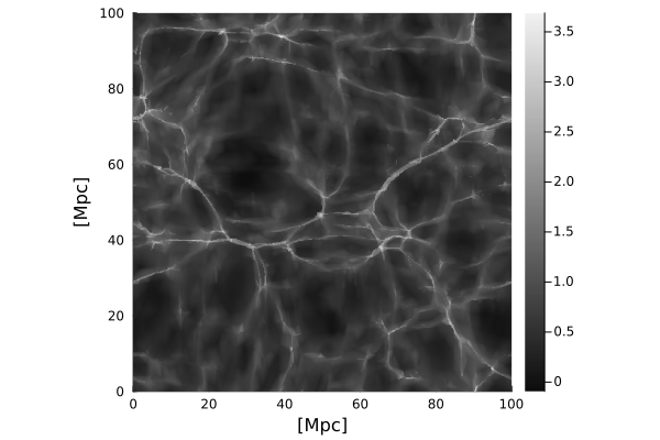
The number of streams follows analogously with numberOfStreams_subbox()-function:
nstreams_field = numberOfStreams_subbox(coords_arr, ps_dtfe_sb)
heatmap(Range, Range, nstreams_field, aspect_ratio=:equal, xlims=(0, L), ylims=(0, L), clim=(1, 7), xlabel="[Mpc]", ylabel="[Mpc]")
Finally, the velocities are evaluated with the velocity()- or velocitySum()-function:
velocitySum_field = velocitySum_subbox(coords_arr, ps_dtfe_sb)We clear the temporary files here. The user might wish to consider storing the estimators for further use.
rm("ps_dtfe", recursive=true)
rm("ps_dtfe_sb.jld2")